load libraries
library(dplyr)
library(sf)
library(ggplot2)Jens Wiesehahn 
Orthoimagery and airborne laser scanning data in Lower Saxony is acquired on a regular basis by LGLN, for many applications the acquisition date is important. We use R to query and plot this information for orthophotos, image-based height models and ALS-based height models.
The State Office for Geoinformation and Land Surveying Lower Saxony (LGLN) provides a lot of its geospatial datasets under open licences. These include orthoimages (DOP), image-based surface height models (bDOM), as well as terrain (DGM) and surface (DOM) models derived from airborne laser scanning (ALS). In recent years the data has been made available as Cloud Optimized GeoTIFFs (COG) and referenced through SpatioTemporal Asset Catalogs (STAC).
We use R to access and explore the acquisition dates of these datasets. The index of available data - stored as a GeoJSON file in a cloud bucket - contains numerous polygons representing image tiles (1 km² or 2 km²) covering Lower Saxony. Each tile contains some basic metadata and links to further metadata as well as links to the image data itself. We fetch the index files for orthoimages (DOP), image-based height models (bDOM) and ALS-based height models (DGM/DOM) to examine acquisition timing.
More information about the data is available at opengeodata.lgln.niedersachsen.de.
Due to phenological effects there are different demands to the data in vegetated areas. For orthophotos, data collection during the leaf-on season is preferred to get information from tree canopy such as vitality and to get better results during image-matching for height model processing. In contrast, terrain models derived from ALS data benefit from leaf-off conditions, when more laser pulses can penetrate the canopy and reach the ground surface.
DOP and bDOM originate from the same underlying imagery, but the available tiles and acquisition dates may differ because bDOM is generated only for a subset of images. Similarly, DGM and DOM are both derived from ALS data, but the available tiles and acquisition dates may differ.
The data is also indexed in as STAC which allows for advanced searching, filtering and processing. It can be e.g. explored via Radiant Earth STAC-Browser.
library(dplyr)
library(sf)
library(ggplot2)# read geojson from cloud bucket
get_data <- function(geojson){
dat <- st_read(geojson) |>
# modify date
mutate(
date = lubridate::ymd(Aktualitaet),
year = lubridate::year(date),
month = lubridate::month(date, label = TRUE),
doy = lubridate::yday(date)
)
return(dat)
}
dop20<- get_data("https://arcgis-geojson.s3.eu-de.cloud-object-storage.appdomain.cloud/dop20/lgln-opengeodata-dop20.geojson")Reading layer `lgln-opengeodata-dop20-rgbi' from data source
`https://arcgis-geojson.s3.eu-de.cloud-object-storage.appdomain.cloud/dop20/lgln-opengeodata-dop20.geojson'
using driver `GeoJSON'
Simple feature collection with 66656 features and 6 fields
Geometry type: POLYGON
Dimension: XY
Bounding box: xmin: 340000 ymin: 5682000 xmax: 676000 ymax: 5980000
Projected CRS: ETRS89 / UTM zone 32Nbdom20<- get_data("https://arcgis-geojson.s3.eu-de.cloud-object-storage.appdomain.cloud/bdom20/lgln-opengeodata-bdom20.geojson")Reading layer `lgln-opengeodata-bdom20' from data source
`https://arcgis-geojson.s3.eu-de.cloud-object-storage.appdomain.cloud/bdom20/lgln-opengeodata-bdom20.geojson'
using driver `GeoJSON'
Simple feature collection with 102979 features and 4 fields
Geometry type: POLYGON
Dimension: XY
Bounding box: xmin: 340000 ymin: 5682000 xmax: 676000 ymax: 5980000
Projected CRS: ETRS89 / UTM zone 32Ndgm1<- get_data("https://arcgis-geojson.s3.eu-de.cloud-object-storage.appdomain.cloud/dgm1/lgln-opengeodata-dgm1.geojson")Reading layer `lgln-opengeodata-dgm1' from data source
`https://arcgis-geojson.s3.eu-de.cloud-object-storage.appdomain.cloud/dgm1/lgln-opengeodata-dgm1.geojson'
using driver `GeoJSON'
Simple feature collection with 63275 features and 4 fields
Geometry type: POLYGON
Dimension: XY
Bounding box: xmin: 342000 ymin: 5682000 xmax: 675000 ymax: 5972000
Projected CRS: ETRS89 / UTM zone 32Ndom1<- get_data("https://arcgis-geojson.s3.eu-de.cloud-object-storage.appdomain.cloud/dom1/lgln-opengeodata-dom1.geojson")Reading layer `lgln-opengeodata-dom1' from data source
`https://arcgis-geojson.s3.eu-de.cloud-object-storage.appdomain.cloud/dom1/lgln-opengeodata-dom1.geojson'
using driver `GeoJSON'
Simple feature collection with 63275 features and 4 fields
Geometry type: POLYGON
Dimension: XY
Bounding box: xmin: 342000 ymin: 5682000 xmax: 675000 ymax: 5972000
Projected CRS: ETRS89 / UTM zone 32NThe data catalog contains information about the acquisition date of images. We can plot this data to get more information about the available images. Acquisition dates for bDOM should be in principle the same as for DOP as the underlying image data is the same, however not all images were processed to bDOM as the necessary data quality (overlap) has not always been fulfilled.
# first and last available acquisition dates
get_timespan <- function(dat){
  min <- dat|> arrange(date) |>  slice(1) |> pull(date)
  max <- dat|> arrange(desc(date)) |>  slice(1) |> pull(date)

  cat("Images available from", format(min), "to", format(max), "\n")
}

plot_distribution <- function(dat){
  dat |>
  ggplot(aes(x = doy)) +
  geom_bar() +
  scale_x_continuous(
    breaks = c(1, 32, 60, 91, 121, 152, 182, 213, 244, 274, 305, 335),
    labels = month.abb,
    limits = c(1, 365)
  ) +
  labs(x = NULL, y = NULL) +
  theme_void() +
  theme(
    axis.text.x = element_text(),
    legend.position = "top"
  )
}Images available from 2012-03-15 to 2025-04-29 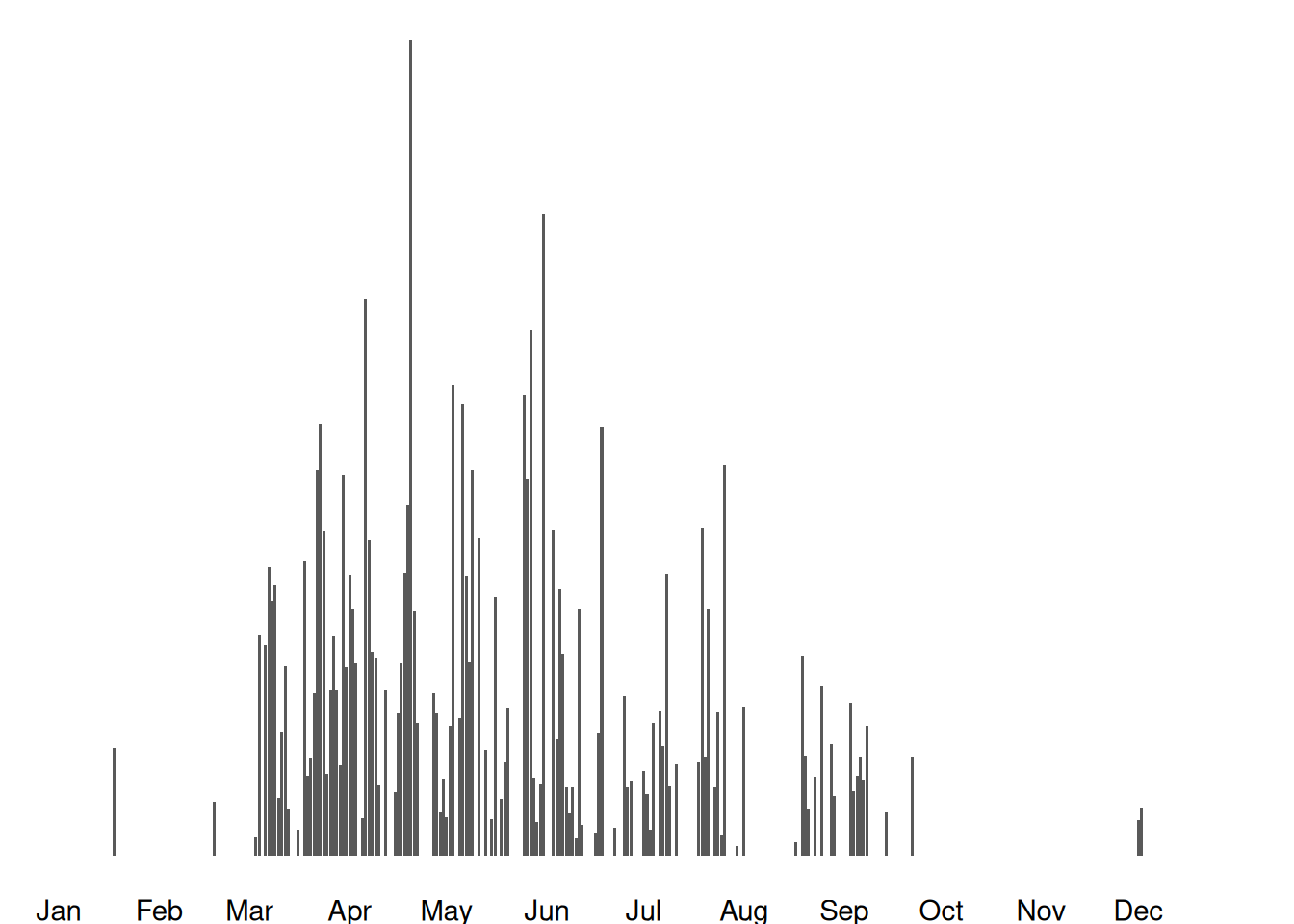
Images available from 2021-03-29 to 2025-04-29 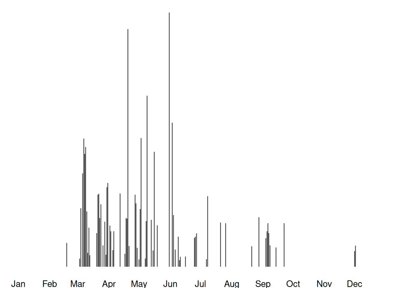
Images available from 2010-05-14 to 2023-09-05 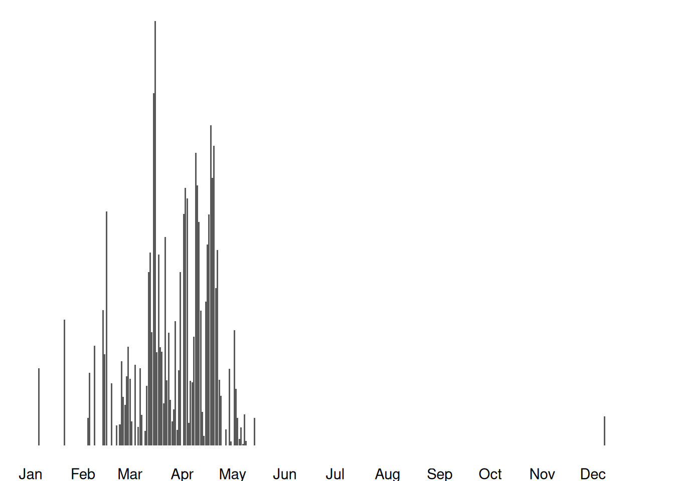
Images available from 2010-05-14 to 2023-09-05 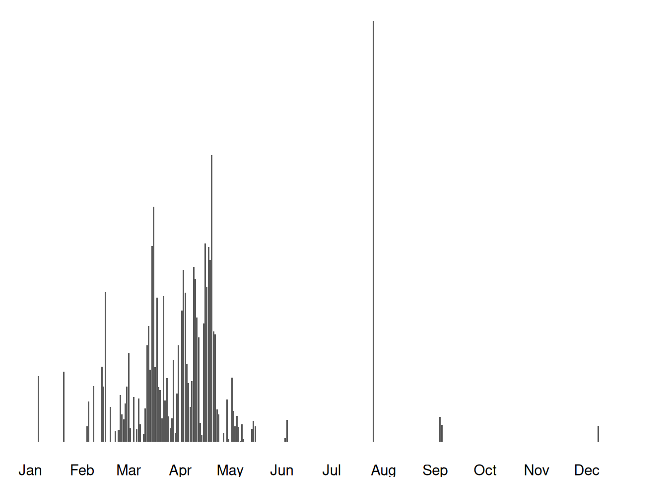
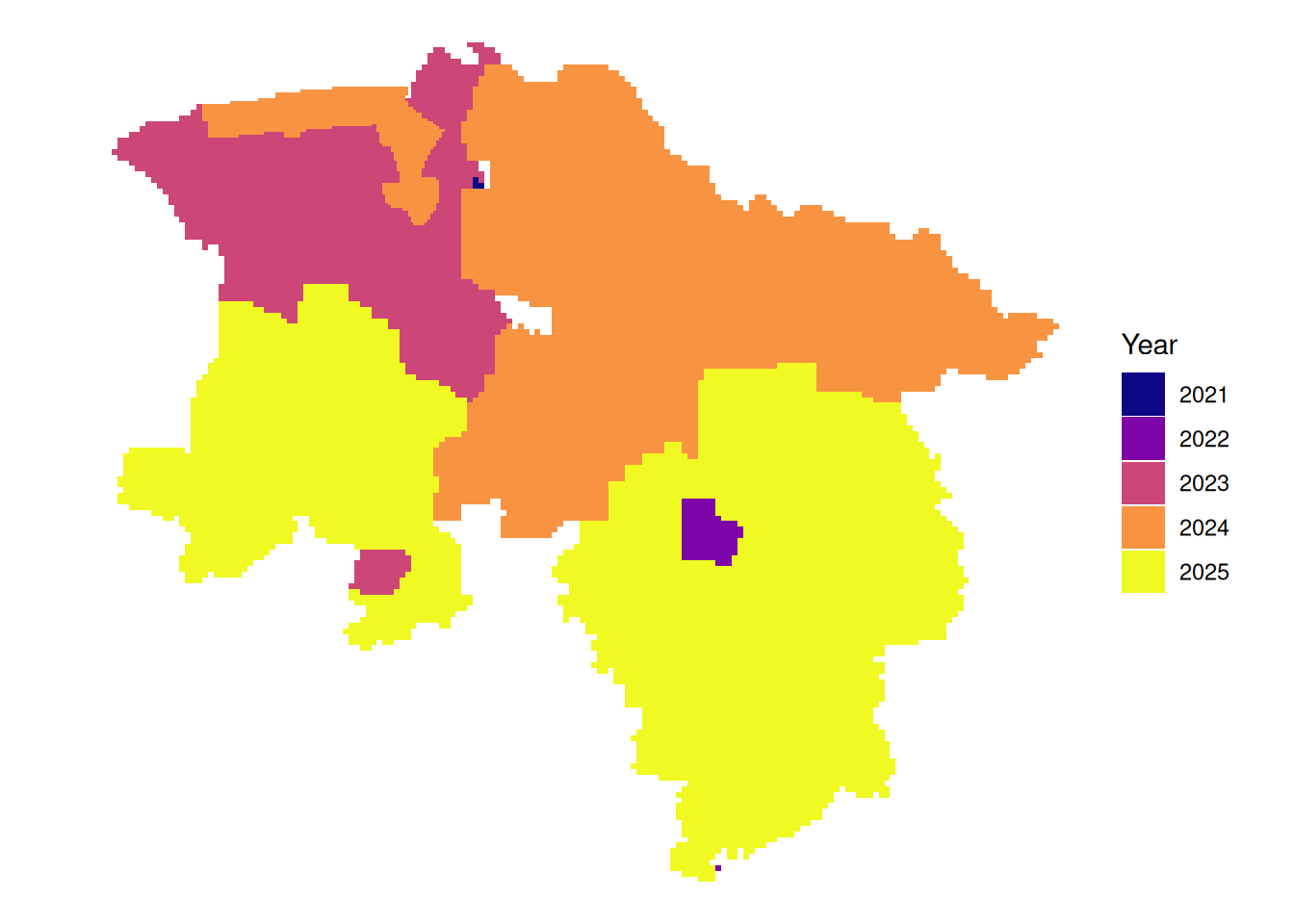
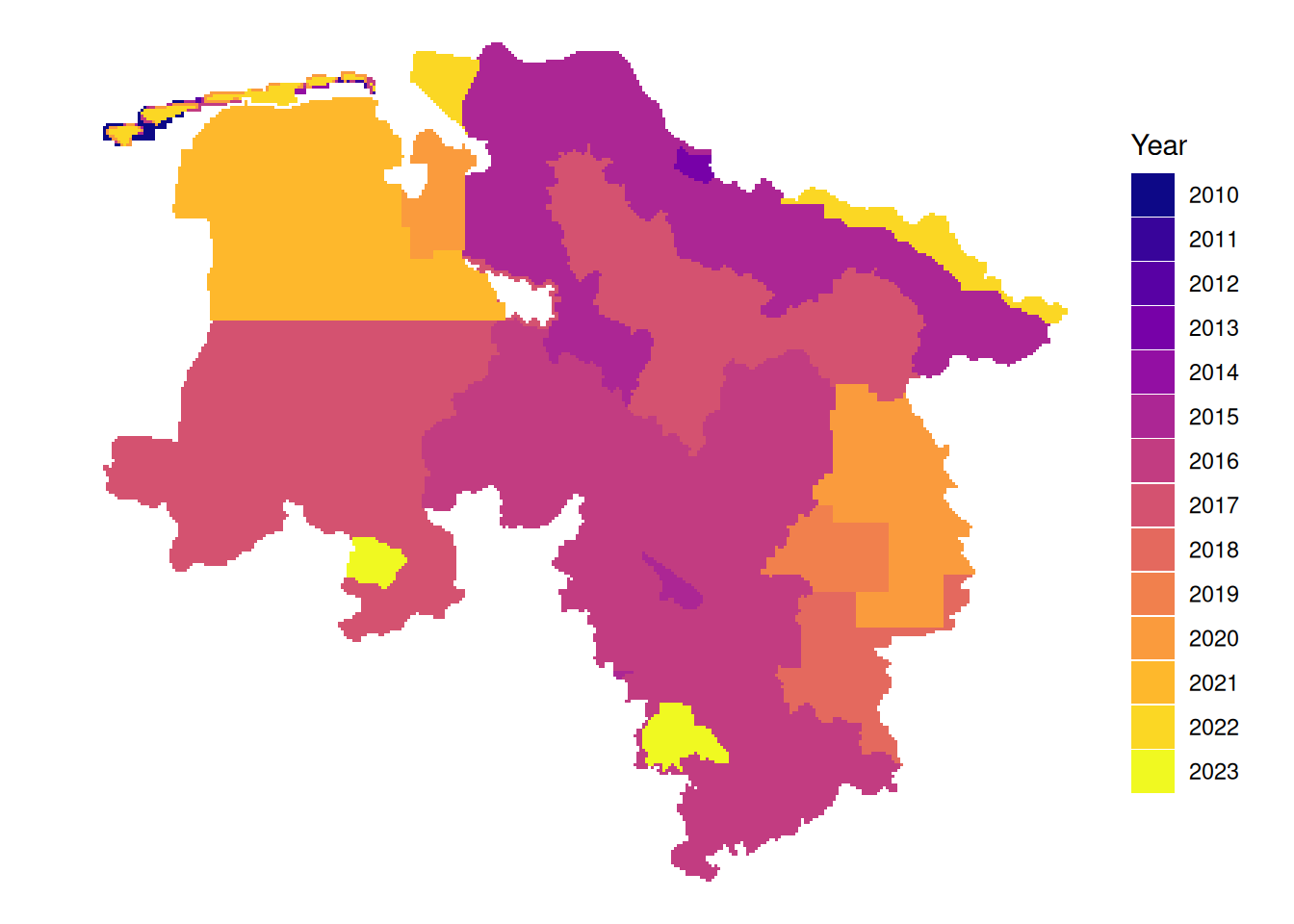
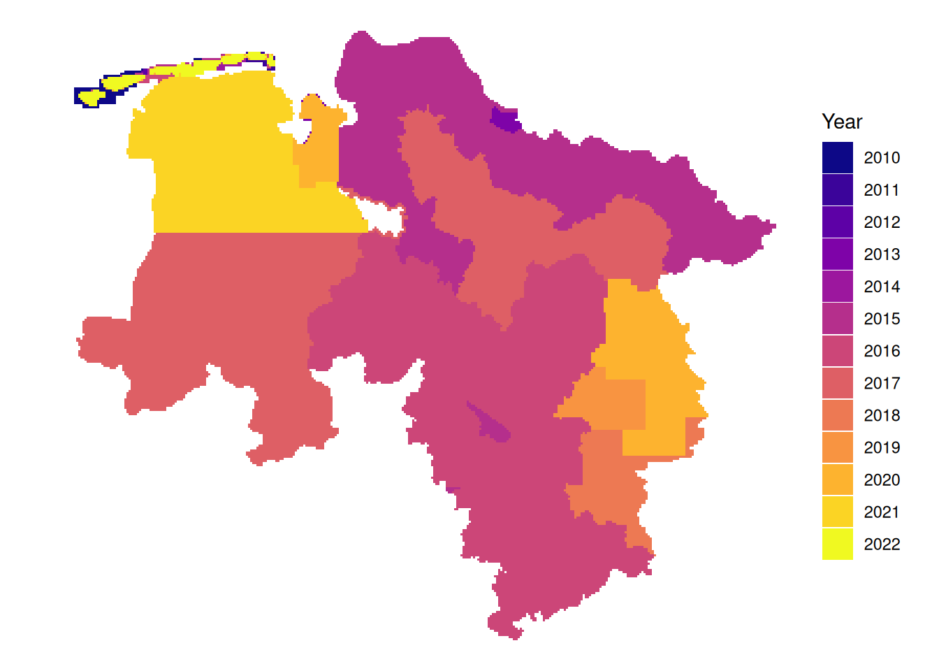
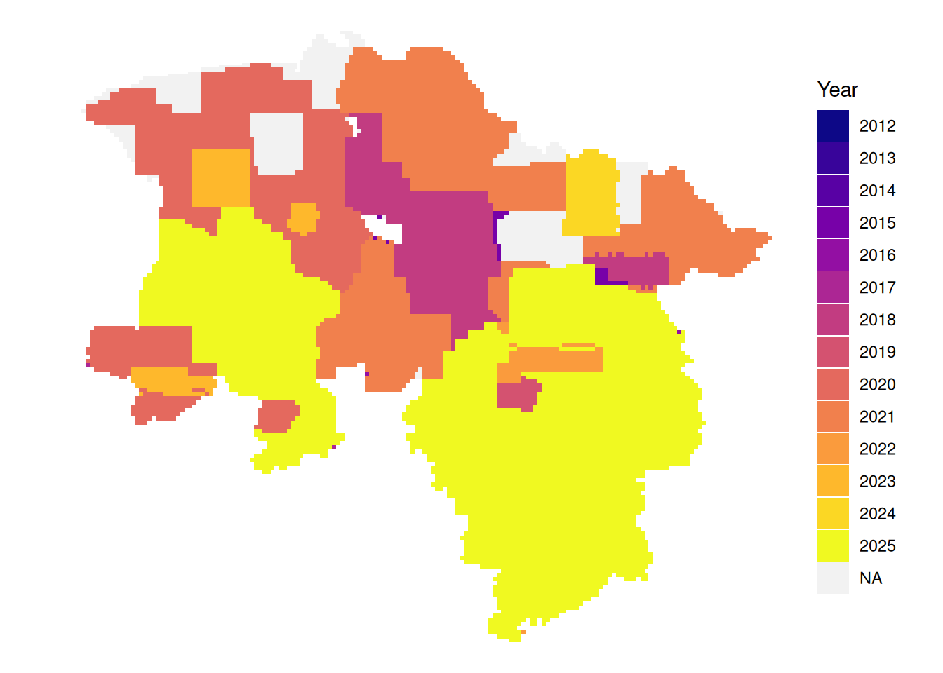
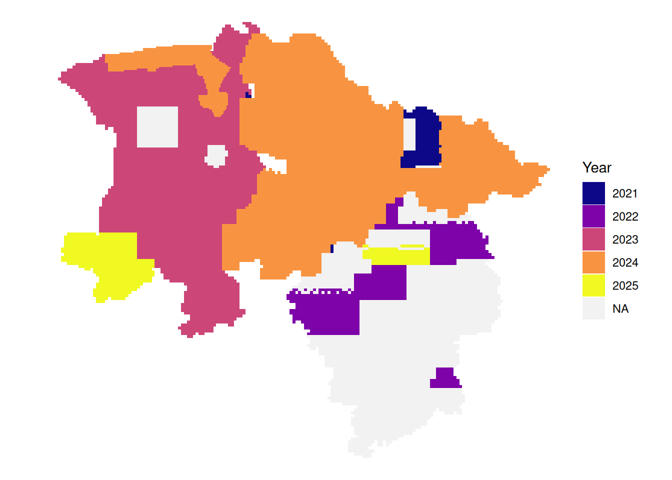
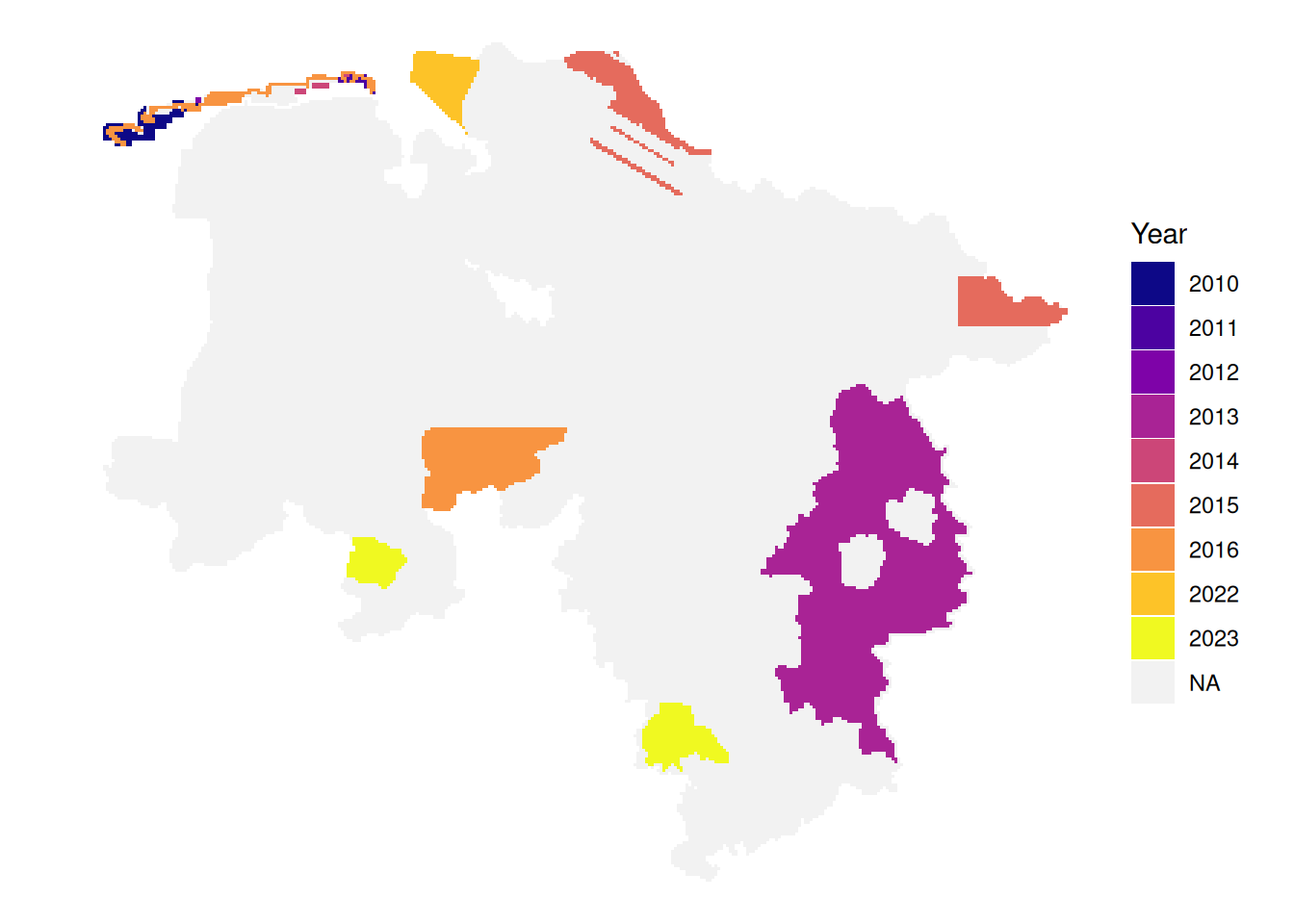
# latest acquisition date per tile
plot_latest <- function(dat){
  dat|>
  group_by(tile_id) |>
  slice_max(date, n = 1) |>
  ggplot() +
    geom_sf(aes(fill = as.factor(year)), color = NA) +
    theme_void()  +
    scale_fill_viridis_d(option = "plasma", name = "Year")
}

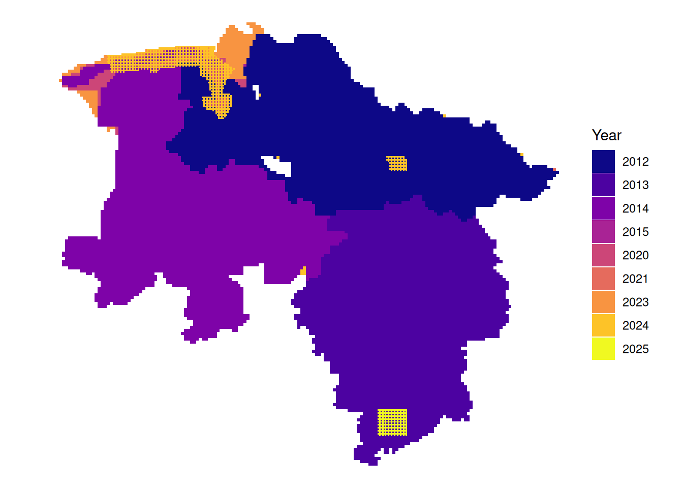
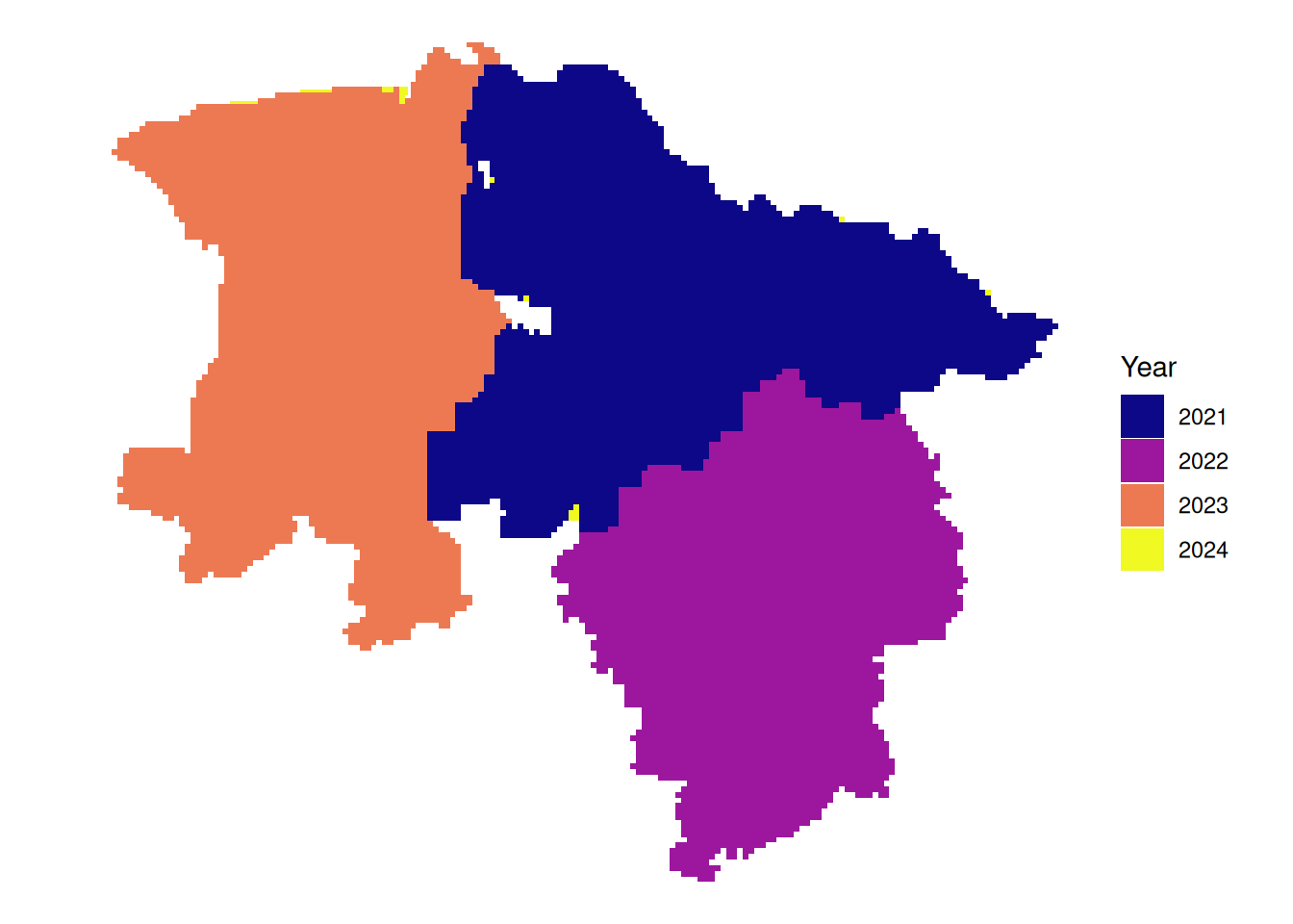
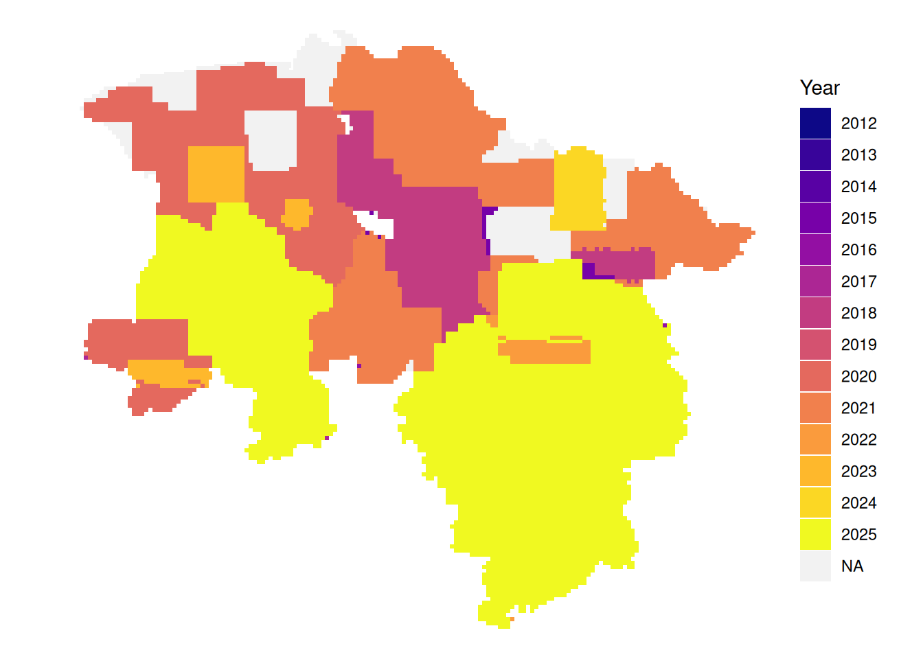
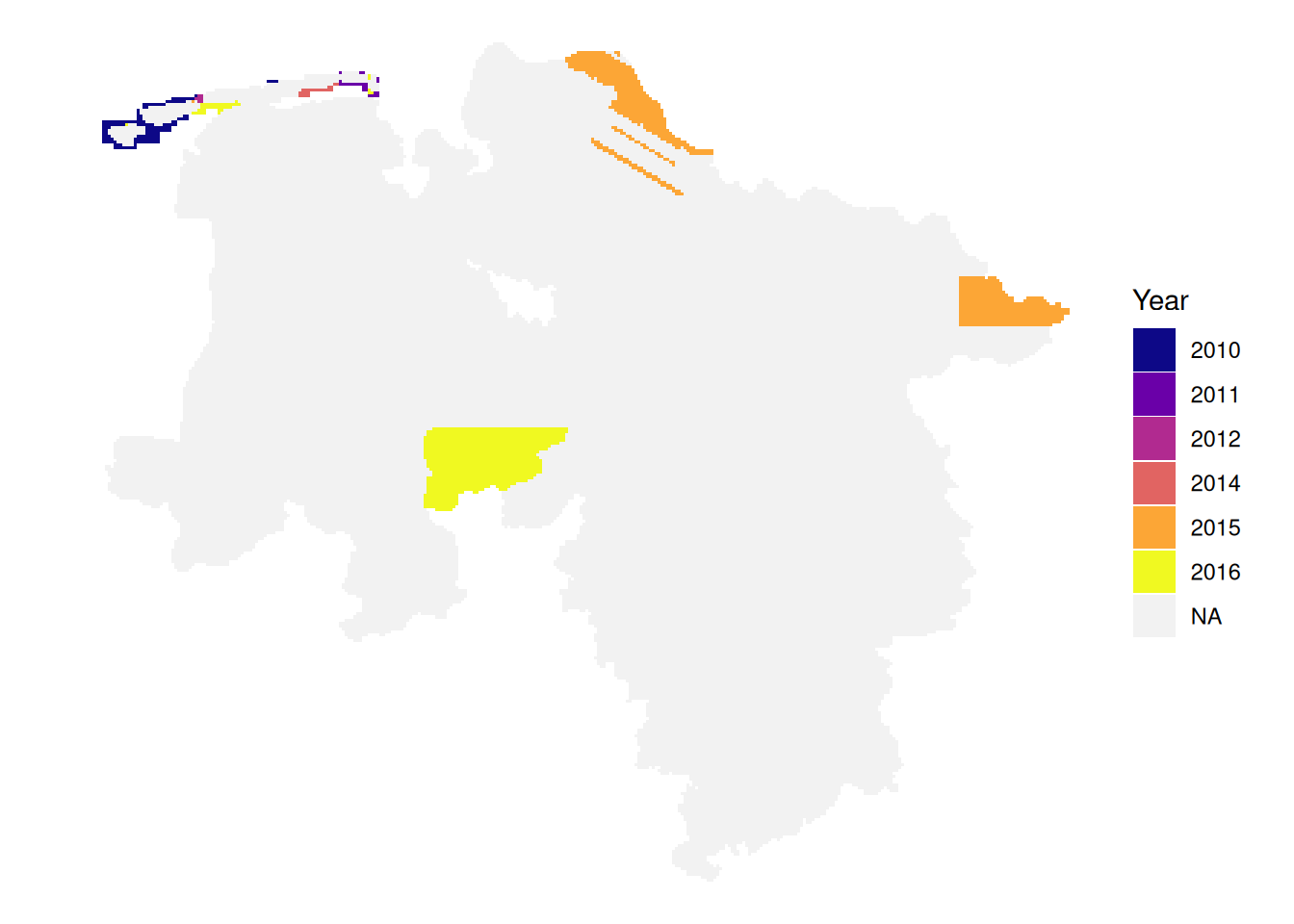
# first acquisition date per tile
plot_first <- function(dat){
  dat|>
  group_by(tile_id) |>
  slice_min(date, n = 1) |>
  ggplot() +
    geom_sf(aes(fill = as.factor(year)), color = NA) +
    theme_void()  +
    scale_fill_viridis_d(option = "plasma", name = "Year")
}
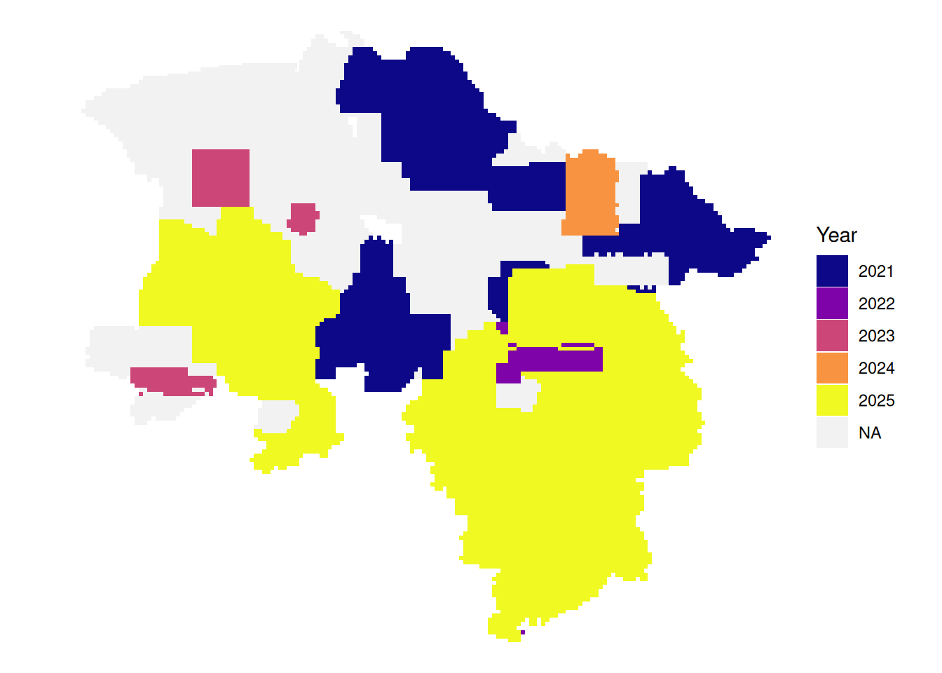
# latest leaf-off data per tile
plot_leafoff <- function(dat){
  dat|>
  mutate(Year = if_else(!between(doy, 115, 315),
                        as.character(year),
                        NA_character_)) |>
  arrange(!is.na(Year), date) |>
  ggplot() +
    geom_sf(aes(fill = Year), color = NA) +
    theme_void() +
    scale_fill_viridis_d(option = "plasma", na.value = "#f2f2f2", name = "Year")
}
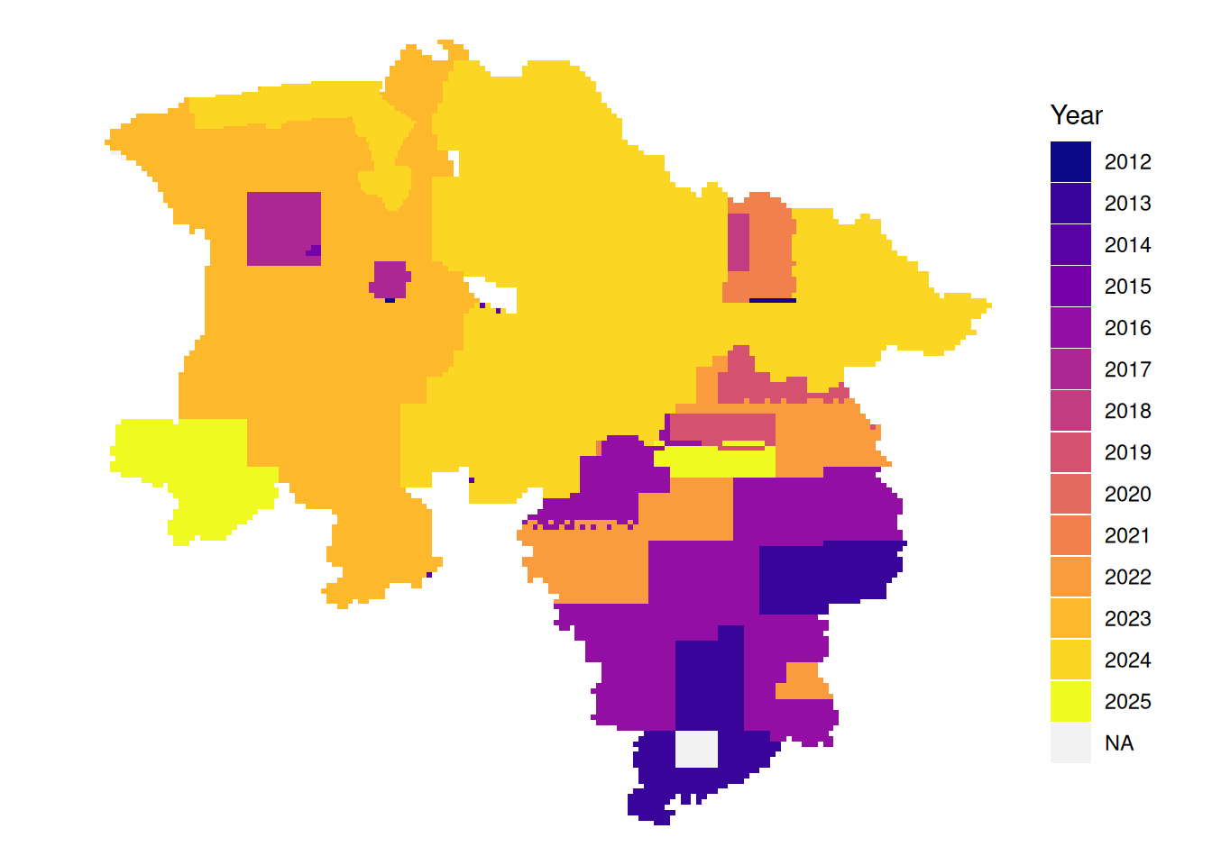
# latest leaf-on data per tile
plot_leafon <- function(dat){
  dat|>
  mutate(Year = if_else(between(doy, 115, 315),
                        as.character(year),
                        NA_character_)) |>
  arrange(!is.na(Year), date) |>
  ggplot() +
    geom_sf(aes(fill = Year), color = NA) +
    theme_void() +
    scale_fill_viridis_d(option = "plasma", na.value = "#f2f2f2", name = "Year")
}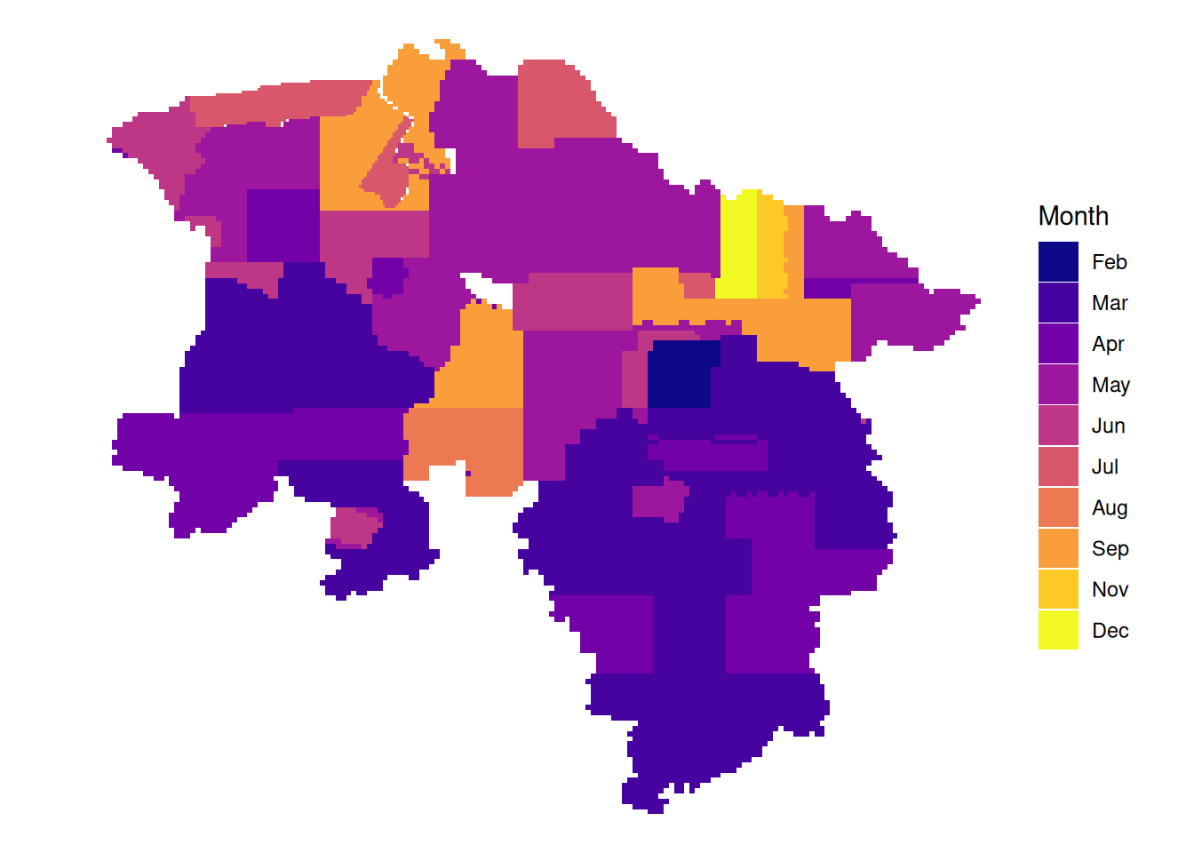

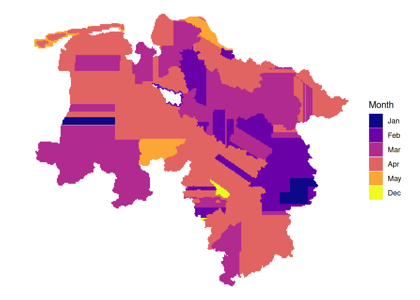
# month of latest data per tile
plot_month <- function(dat){
  dat|>
  group_by(tile_id) |>
  slice_max(date, n = 1) |>
  ggplot() +
    geom_sf( aes(fill = month), color = NA) +
    theme_void()  +
    scale_fill_viridis_d(option = "plasma", name = "Month")
}
  Jan   Feb   Mar   Apr   May   Jun   Jul   Aug   Sep   Oct   Nov   Dec
328 164 15258 15078 16146 6989 7336 2834 2271 0 107 145 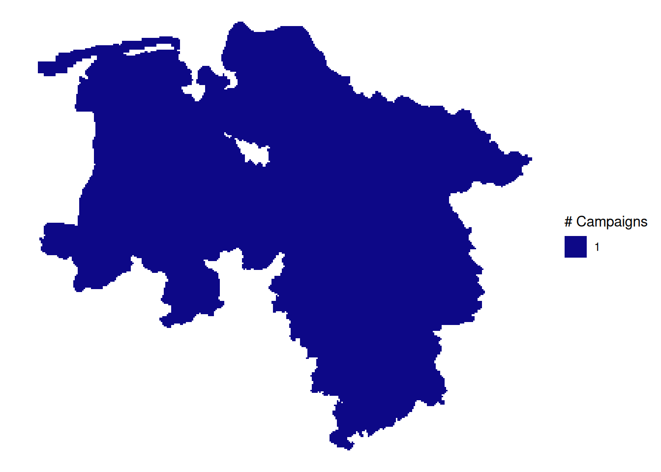
  Jan   Feb   Mar   Apr   May   Jun   Jul   Aug   Sep   Oct   Nov   Dec
0 656 34077 20160 24408 9960 4568 1932 6210 0 428 580 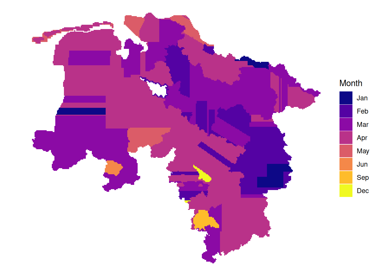
  Jan   Feb   Mar   Apr   May   Jun   Jul   Aug   Sep   Oct   Nov   Dec
1400 6971 19012 28407 2265 257 4365 0 433 0 0 165 
  Jan   Feb   Mar   Apr   May   Jun   Jul   Aug   Sep   Oct   Nov   Dec
1400 6971 19012 28407 2265 257 4365 0 433 0 0 165 # month of latest data per tile
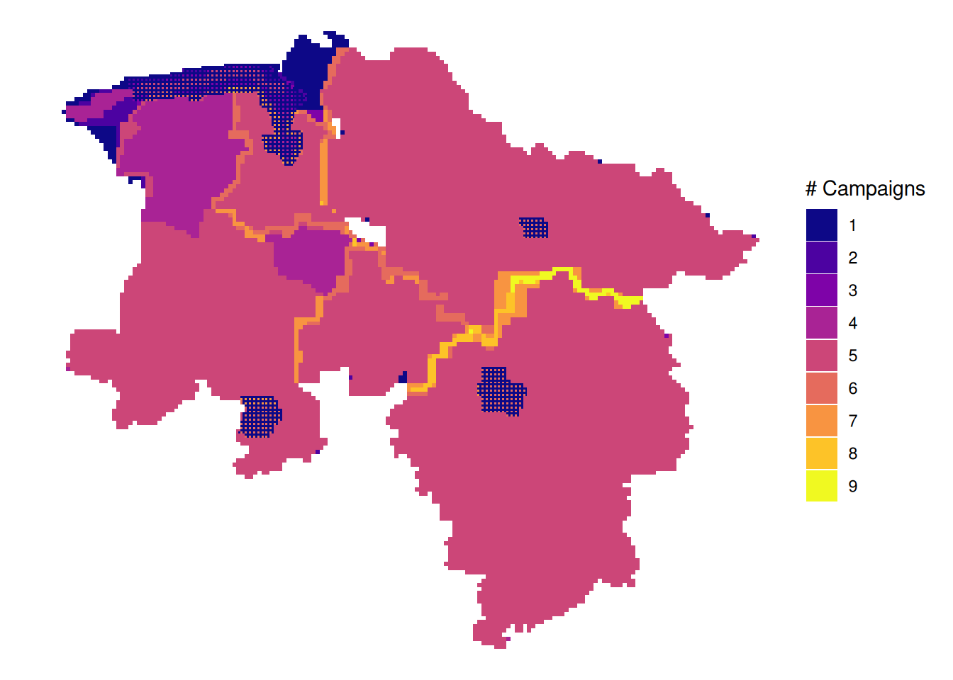
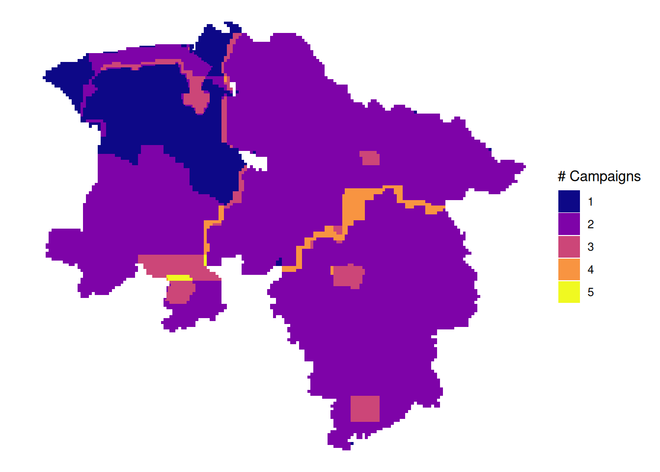
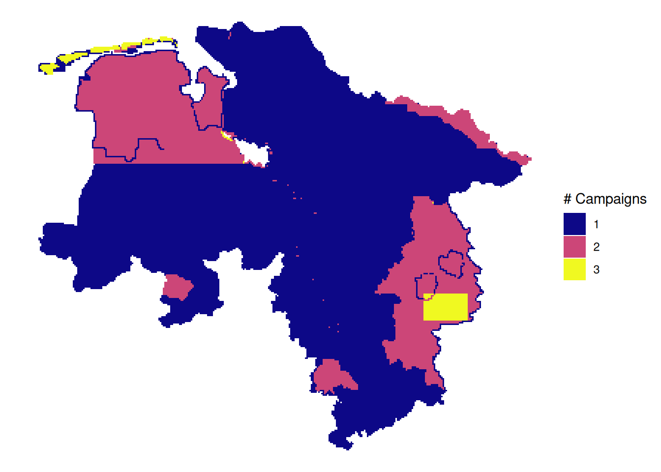
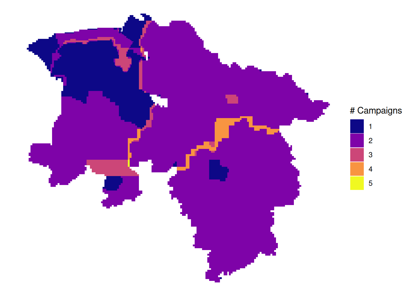
plot_number <- function(dat){
dat|>
st_drop_geometry() |> # Work with data first
group_by(tile_id) |>
summarise(n = n()) |>
left_join(dat|> select(tile_id) |> distinct(), by = "tile_id") |>
st_as_sf() |>
ggplot() +
geom_sf( aes(fill = as.factor(n)), color = NA) +
theme_void() +
scale_fill_viridis_d(option = "plasma", name = "# Campaigns")
}